Goals. The goal of this computer lab is that you train a segmentation model, fitting its parameters to empirical data, and evaluate its performance. The model that you will train is the Retention&Recognition model (RnR henceforth). You can find a short description of the model in @alhama2015should and in the slides in the materials/ directory. We will use the data and evaluation procedures described in @frank2010modeling.

Requirements. The lab uses Python 3 with the libraries matplotlib and numpy. If you don’t have these libraries installed you can install them using pip or conda. In case you are not very familiar with drawing plots in python, you might find this matplotlib gallery helpful.

Materials All materials can be found in the materials/ directory; the subdirectory data contains three files, each one containing human responses for each of the three experiments described in @frank2010modeling. In the src directory you find the following python files:

• models.py contains implementations of the example model (PolynomialModel) and a wrapper for the Retention&Recognition model (RnRModel).
• optimization.py contains the two optimization algorithims we use in this lab: grid search and hill climbing.
• experiment.py contains the code to generate the stimuli used by @frank2010modeling, and to load their experimental results.
• RnR.py implements the Retention&Recognition model. You don’t need to understand the details.

You don’t need to understand what happens in experiment.py and RnR.py, only how you can use it. You do, however, need to to understand what the first two files are doing.

Introduction

When learning a language, infants learn to identify word boundaries in the streams of speech sounds they hear. Artificial language learning paradigms have been used to study how they can do this. Typically, subjects are exposed to an artifical stream of speech sounds containing statistical regularities. After listening to this for a while, they are presented with a sound and have to decide whether it is a word or a partword.

In this computer lab we look at a computational model of precisely this: segmentation in artificial language learning: the Retention&Recognition (RnR) model [@alhama2015should;@alhama2017segmentation]. This is a probabilistic segmentation model that tries to break a given stream of syllables into segments. The model works based on two probabilities: the recognition probability and the retention probability. The recognition and retention probabilities of a segment $s$ are computed as follows:

As you can see, the model involves four parameters $A,B,C$ and $D$ that should be fitted to empirical data. Computational models normally include a set of free parameters. The behaviour of the model changes depending on the values of such parameters. Hence, after choosing a computational model, the next step is to set the parameters of the model so that the behaviour/output of the model is consistent/similar to the phenomenon that is being modelled. This is what we call training or fitting the model. To explain this in more detail, we are first going to train an example model: a polynomial of degree 2, where it is easier to see what is going on. After that, we return to the RnR model.

Model fitting

An example model: a polynomial

To get started, we are going to model the relation between two variables $x$ and $y$. We have a set of $n$ observations $(x_i, y_i)$ and now want to formulate a model that predicts the value of $y$ for a given $x$. In other words, we want to fit a curve through the observed points $(x_i, y_i)$. After long deliberation we decide that the curve should be a polynomial of degree 2. The predicted value $y_\text{pred}$ for a given $x$ then takes the form

where $A$, $B$ and $C$ are the parameters of the model. (Since the prediction depends on the parameters, it would be better to write $y_{\text{pred}}(x \mid A, B, C)$)

Now we have to choose the values of these parameters in order to get a curve that best approximates the data points. But what do we mean by best approximation? We formally define this using an objective function. This function measures either how well your predictions fit the observed data, or how poorly (then it’s often called a cost function). During the training phase you want to maximize or minimize the objective funciton. In other words, we want to find the parameters values that result in the best between predictions and observations, as measured by the objective function.

In this example, we can define the objective function as the (mean absolute) difference between observed values $y_i$ and the values $y_{\text{pred}}(x_i)$ predicted by our polynomial model. This would be a cost function which we want to minimize. For the mathematically inclined, you could define it as follows:

One thing to consider is that, depending on the data points, it is not always possible to find the set of parameters that gives us an objective function with minimum possible value (zero in this case).

Grid search

Now, if we have the model, the objective function, and the data points, how can we find the best set of values for the parameters? The algorithms that are used to find the best set of values for the parameters of a model are called optimization algorithms. Here, we look at two different optimization algorithm: grid search and hill climbing.

One way to find the optimal parameter setting is to compute the objective function for all possible equidistant combinations of different values for the parameters, and then choose the combination that gives us the lowest cost (the output of the cost function). This method is called grid search.

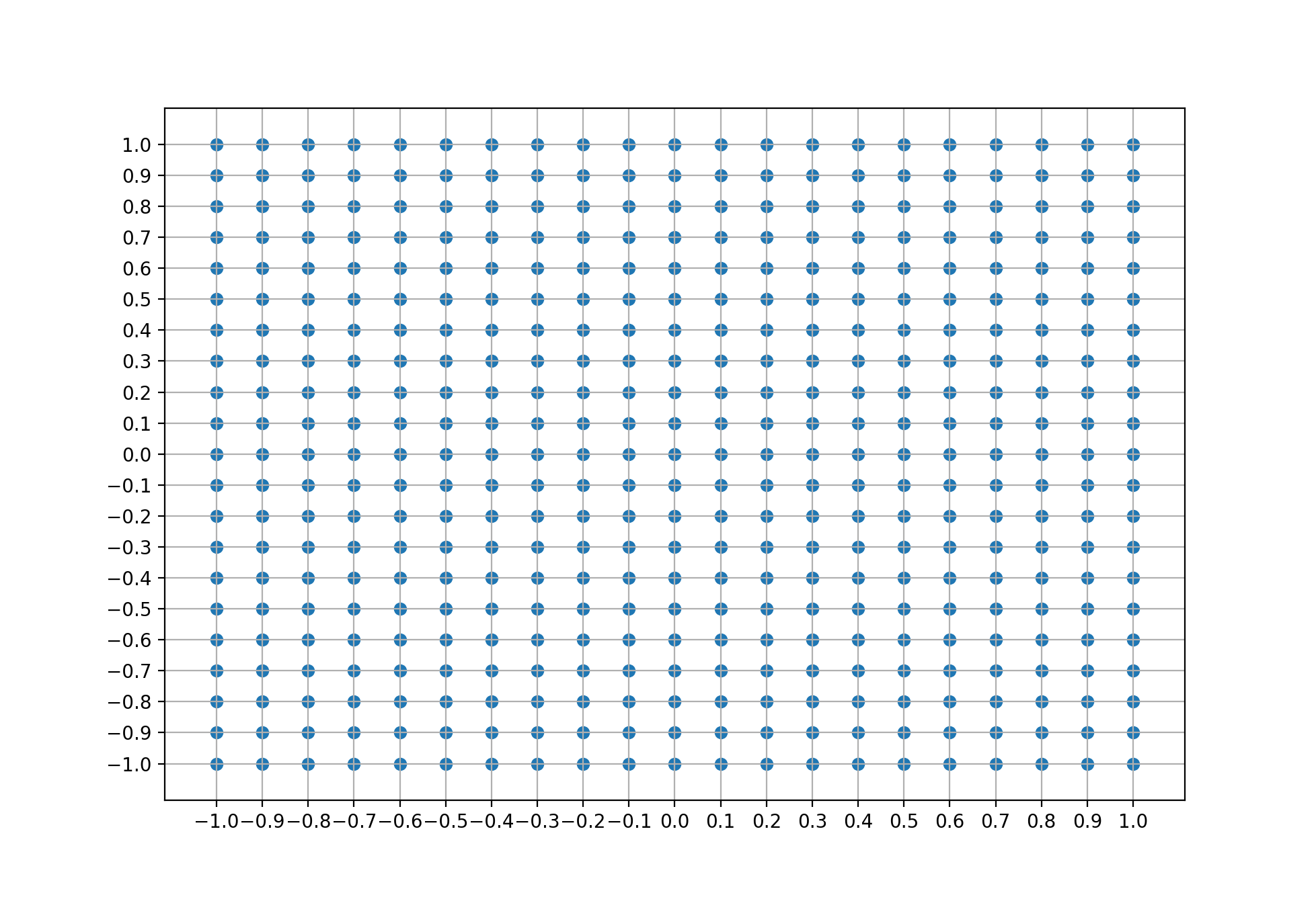
In the example model, set $C$ to a random value, and assume $A$ and $B$ can be any real value in the range $[-1,1]$. We have to pick a step size, let’s say 0.1. (Since there are indefinite possible values we pick a step size in order to pick a sample.) Thus we would have 21 possible values for both $A$ and $B$: $\{-1,-.9,-.8,0.7,...,0,.1,.2,...,.9,1\}$ If we take all possible combinations, we would have $21 \times 21$ parameter settings. This gives us the grid in the figure below.

from polynomial import PolynomialModel, generate_training_data
model = PolynomialModel(A_init=2, B_init=3, C_init=.75)
data = generate_training_data(num_datapoints=30)

cost_matrix, domains = grid_search(model, data, step_size=.05, optimize=['A', 'B'])

Hill climbing

There are several methods that help us avoid exploring the whole space of the parameter values, using greedy decisions to directly explore the space in the direction that is more probably closer to the minimum point. One of those is the hill climbing algorithm.

Hill climbing is a so called local search algorithm. The idea behind it is that you start from a random point (where each point is a possible solution for the problem), then you decide in which direction you should change the parameters based on the value of the cost function at the current point and its neighbours. Greedily, in each iteration, you choose the next point to be where the cost function is the lowest.

There exist different versions of this algorithm. Here, we will implement simple hill climbing. Informally, you can think about simple hill climbing as if you were lost in some huge hilly landscape and your goal is to find the highest point. If you follow this algorithm, you would make a step from where you are, in one random direction, and see if you have moved higher. If so, you choose your next random direction from this point; if, instead, the landscape goes down, then you go back where you were and choose another random direction.

The RnR model

Now that you know how you can fit a model using grid search and hill climbing, we return to the Retention&Recognition model. An implementation of the RnR model is provided, and your task is to fit the parameters of this model (train the model) on the dataset that is provided.

The data

The dataset we use comes from @frank2010modeling. The authors three experiments to study how different factors affect word segmentation. These factors are:

• Experiment 1: sentence length\ In this experiment the number of tokens (100) and the size of the vocabulary (6) are fixed. The sentence length is set to be 1, 2, 3, 4, 6, 8, 12 or 24.

• Experiment 2: number of tokens\ In this experiment the size of the vocabulary (6) and sentence length (4) are fixed. The total number of tokens in the input stream is set to be 48, 100, 300, 600, 900 or 1200.

• Experiment 3: size of the vocabulary\ In this experiment the number of tokens (600 / vocabulary_size) and the length of the sentence (4) are fixed. The vocabulary size is set to be 3, 4, 5, 6 or 9.

In each experiment the input stream is generated pseudo-randomly to satisfy the specified criteria. After being exposed to this stream, the participants answer a 2-alternative forced choice test in which they choose between words and partwords. These responses are collected in three data files in the materials/data directory. The file experiment.py contains a Python class that can load all the human responses:

from experiment import Experiment
# You can set experiment_id to 1, 2, or 3
experiment = Experiment(experiment_id=1, data_dir='../data/')
results = experiment.results

If you run into problems when trying to import experiment.py from outside the materials/src directory, first add the directory to your path:

import sys
sys.path.append('../relative/path/to/materials/src')

If all that worked, the object results has now loaded and processed human responses. It has some useful properties:

• results.data is a list of tuples containing the condition, subject, and if he/she was correct or not

• results.performance is performance of each subject for each condition. You can also plot the performance of participants in the experiment using experiment.plotPerformance().

• results.avg_performance is average performance of all subjects for each condition

• results.std_performance is standard deviation of performance of all subjects on each condition

Every experiment has several conditions, which are stored in experiment.conditions. You can also find the stimuli (and the concatenated stream) there. For example:

experiment = Experiment(experiment_id=1, data_dir='../data/')
condition = experiment.conditions[1]
print(condition.stimuli)
print(condition.stream)

The model

As explained in the introduction, the RnR model is a probabilistic segmentation model with four free parameters: $A, B, C$, and $D$. The file models.py contains (a light wrapper around) an implementation of the RnR model. The following snippet shows how you can instantiate the RnR model and see the words it memorizes:

from models import RnRModel
model = RnRModel(A=0.04, B=0.3, C=0.3, D=0.3, nmax=4)

for condition in experiment.conditions.values():
    # Memorized words per length
    stream = condition.stream
    subjective_frequencies = model.memorizeOnline(stream)

    # Extract the words only
    words = list(flatten([f.keys() for f in subjective_frequencies.values()]))
    print(condition, '\n', words, '\n')

In order to test the performance of the model, after each input stream, a list of pairs of sequences consisting of one word and one partword will be given to the model, and it has to decide which of the sequences is more likely to be a word. These test pairs are stored in condition.test. The output of the RnR model consists of a memory of segments, together with their subjective frequencies. In order to convert that output to the probabilities of choosing a test item, we use the Luce rule, which states that, given two alternative options $s_1$ and $s_2$ to choose from (sequences in our case), the probability to choose one over the other is:

where score is, in the case of the RnR model, a subjective frequency. In the code, we call the Luce choice rule as follows:

prob_1, prob_2, chosen = model.luce(word_1, word_2)

Training

Now that you know what does it mean to fit a model to some data, you are ready to train the RnR model. In the RnR model, there are 4 parameters to be tuned $(A, B, C, D)$, and they all should be in the range of $(0,1)$. The goal is to set these parameters in a way that this model behaves as similar as possible to humans in doing the segmentation task. The objective function is Pearson’s $r$, which computes the correlation between the performances of the model and the average performances of humans for different conditions.

Evaluating