3. Hopfield Networks#

This notebook is part of a larger effort to offer an approachable introduction to models of the mind and the brain for the course “Foundations of Neural and Cognitive Modelling”, offered at the University of Amsterdam by Jelle (aka Willem) Zuidema. The notebook in this present form is the result of the combined work of Iris Proff, Marianne de Heer Kloots, and Simone Astarita.

Instructions#

The following instructions apply if and only if you are a student taking the course “Foundations of Neural and Cognitive Modelling” at the University of Amsterdam (Semester 1, Period 2, Year 2022).

Submit your solutions on Canvas by Tuesday 22th November 18:00. Please hand in the following:

A copy of this notebook with the code and results of running the code filled in the required sections. The sections to complete all start as follows:

### YOUR CODE HERE ###

A separate pdf file with the answers to the homework exercises. These can be identified by the following formatting, where n is the number of points (out of 10) that question m is worth:

Homework exercise m: question(s) (npt).

Introduction#

In the previous labs we looked at models of single neurons. Starting from the Hodgkin-Huxley model, the models successively abstracted away from actual neurons, with the McCulloch-Pitts neuron as the most abstract model we have seen. This week, we see what happens if artiﬁcial neurons are connected to form networks.

We will need the numpy, pandas, matplotlib and imageio libraries, as well as some functions that are defined in the cell below.

!apt install subversion           # for downloading folder from GitHub

import numpy as np                # for algebra
import pandas as pd               # for data manipulation
import matplotlib.pyplot as plt   # for plotting
import imageio                    # for loading image files

# helper functions
def bwcolor(pattern):
    return np.tile(np.array(pattern.T < 1), reps=(3,1,1)).astype('float32').T

def plot_image(pattern):
    plt.imshow(bwcolor(pattern))
    plt.xticks([])
    plt.yticks([])
    plt.show()
    
def plot_patterns(input_patterns, output_patterns, patterns_to_store):
    # convert patterns to images
    pixels = len(list(patterns_to_store.values())[0]) - 1
    shape = (np.sqrt(pixels).astype('int'), np.sqrt(pixels).astype('int'))
    input_patterns = {d: input_patterns[d][:pixels].reshape(shape)
                     for d in input_patterns}
    output_patterns = {d: output_patterns[d][:pixels].reshape(shape)
                     for d in output_patterns}
    patterns_to_store = {d: patterns_to_store[d][:pixels].reshape(shape)
                     for d in patterns_to_store}
    
    # create plot
    fig, axs = plt.subplots(3, len(patterns_to_store))
    
    for i, d in enumerate(sorted(patterns_to_store)):
        axs[0, i].imshow(input_patterns[d], cmap="binary_r")
        axs[0, i].set_xticks([])
        axs[0, i].set_yticks([])
        axs[1, i].imshow(output_patterns[d], cmap="binary_r")
        axs[1, i].set_xticks([])
        axs[1, i].set_yticks([])
        axs[2, i].imshow(patterns_to_store[d], cmap="binary_r")
        axs[2, i].set_xticks([])
        axs[2, i].set_yticks([])
    
    plt.show()
    
def add_noise(pattern, noise_rate):
    noise = (np.random.uniform(0, 1, size=len(pattern)) > noise_rate) * 2 - 1
    noisy_pattern = pattern * noise
    return noisy_pattern
    
def sign(z):
    if z == 0:
        return 1
    else:
        return np.sign(z)

1. Definition of Hopfield networks#

We will study Hopﬁeld networks (or Hopfield nets), which are networks with connections in both directions between all pairs of distinct neurons \((i, j)\). So there is a weight \(w_{ij}\) associated to the connection from \(i\) to \(j\) and a weight \(w_{ji}\) for the connection from \(j\) to \(i\). Moreover, in a Hopﬁeld net it holds that \(w_{ij}\) = \(w_{ji}\) , thus the weights are symmetrical.

Recall from the lecture that the activation (or value) \(y_i\) of a McCulloch-Pitts neuron is a function of (the weighted sum of) the inputs \(x_j\) it receives from other neurons. In a Hopfield net, the total input a neuron receives is

\[ s_i = \sum_{j \neq i} w_{ji} \cdot x_j + \theta_i, \label{eq:neuron_input} \tag{1} \]

where \(\theta_i\) is the bias for a single neuron¹. The activation \(y_i\) is calculated from \(s_i\) using the sign function as the activation function, which evaluates to \(+1\) for inputs \(\geq 0\) and to \(-1\) for inputs \(< 0\):

\[\begin{split} \begin{equation} \tag{2} y_i = \text{sign}{(s_i)} = \begin{cases} +1 & \text{if } s_i \geq 0 \\ -1 & \text{if } s_i < 0 \end{cases} \label{eq:activation} \end{equation} \end{split}\]

In Hopfield networks, we are interested in how the activation of the neurons changes over time. It would therefore be better to write \(y_i^{(t)}\) for the value of neuron \(i\) at time \(t\). Note that the inputs \(x_j\) that a neuron receives are the outputs \(y_j^{(t-1)}\) of other neurons at the previous time step. Using \(y_j^{(t-1)}\) instead of \(x_j\) in \(\eqref{eq:neuron_input}\) and \(\eqref{eq:activation}\) gives the following formula for the activations in a Hopfield net:

\[ y_i^{(t)} = \text{sign}{\Big( \sum_{j \neq i} w_{ji} \cdot y_j^{(t - 1)} + \theta_i \Big)} \label{eq:activation_t} \tag{3} \]

Starting from an initial state \((v_1^{(0)}, ..., v_n^{(0)})\) we can then iteratively calculate the new activation or state of the neuron in the next time step. This can give rise to different kinds of dynamics. A neuron \(i\) is called stable at time \(t\) if its value doesn’t change: \(y_i^{(t)} = y_i^{(t-1)}\). A Hopfield net is called stable if all of its neurons are stable. In that case we also say that the network converged to the stable state.

In this lab we will first look at the different dynamics that can occur when updating the state of the network over time. Next, we will see how we can update the weights of the network and use that to model an associative memory. We often drop the time \(t\), and assume that all the thresholds \(\theta_i\) are \(0\), i.e., we use \(y_i\) instead of \(y_i^{(t)}\), and \(\theta_i = 0\) for all \(i\).

Homework exercise 1: is a Hopfield network a recurrent neural network? (0.5)

¹ You can also think of \(\theta_i\) as a threshold. Using the activation function, equation \(\eqref{eq:activation}\) says that \(y_i = 1\) if \(\sum_{j \neq i} w_{ji} x_j \geq - \theta_i\) (if the weighted sum of the inputs exceeds the threshold \(-\theta_i\)) and \(y_i = -1\) otherwise.

2. Activations in a Hopfield network#

There are two ways to update the state of a Hopfield network. In an asynchronous update, we randomly pick a single neuron at a time and calculate its new activation using equation \(\eqref{eq:activation_t}\). In a synchronous update, all neurons are updated at the same time. It can be proven that if the net is symmetric, i.e. \(w_{ij} = w_{ji}\) for all \(i,j\), then the state of the network will converge to a stable point², which is a local minimum of the following energy function:

\[ E = -\frac{1}{2} \sum_{i,j} w_{ij} y_i y_j = -\frac{1}{2} \mathbf{y}^T\mathbf{Wy}\ . \]

² See Theorem 2, page 51, Kröse & van der Smagt (1996).

2.1 Asynchronous updates#

Consider the network given in the following figure:

ICCN-drive-steps

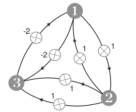
We study how the state of the network changes if we iteratively update its state in an asynchronous fashion. For this, we will use the run_hopfield function defined in the next cell. Instructions on how to use the function follow below.

def run_hopfield(hopnet, pattern, stepbystep=False, 
                 shape=None, maxit=100, replace=True):
    """
    This function computes the activation of a Hopfield network, 
    given the input arguments hopnet (a matrix of weights defining 
    the Hopfield network) and pattern (an array specifying the 
    input pattern / initial state). The output is the network’s
    state after converging (or after the max. nr. of iterations).
    """
    if stepbystep == True:
        # print the network weights and input pattern
        print("weights = ")
        print(hopnet)
        print("input pattern = ", pattern)
        plot_image(pattern.reshape(shape) != 1)
        input()
    
    y = np.copy(pattern)
    n_nodes = len(pattern)
    converge = False

    for it in range(0, maxit):
        
        # asynchronous updating
        if it % n_nodes == 0:
            if (replace == False and converge == True):
                print('Reached a stable state.')
                break
            else:
                # randomly choose the order of updating the n nodes
                order = np.random.choice(range(0, n_nodes), 
                                         size=n_nodes,
                                         replace=replace)
                converge = True
        
        # i = which node to update
        i = order[it % n_nodes]
        
        # y[i] = current value of that node
        yi_old = y[i]
        
        # new value of node i = sign of the dot product of i’s weights and y
        z = hopnet[:,i] @ y
        y[i] = sign(z)
        
        if yi_old != y[i]:
            converge = False
        
        if stepbystep == True:
            # print the update
            print('iter ', it+1)
            print('pick neuron ', i)
            print('input to this neuron ', z)
            print('output of this neuron ', y[i])
            print('new state ', y)
            
            # plot new state
            plot_image(y.reshape(shape) != 1)
            inpt = input()
            if inpt == 'q':
                print('Stopped after', it+1, 'iterations.')
                break
            
    return y

The code in the next cell creates a Hopfield net by defining a weight matrix.

weights = np.array([[0, 1, -2], 
                    [1, 0, 1], 
                    [-2, 1, 0]])

Next, we can ‘run’ several updates of the network. In the next code block, we specify the initial state and can then call the function run_hopfield.

If the argument stepbystep=True is passed, the output is printed step by step. maxit specifies the number of iterations. Running the code block should result in the following output:

weights = 
[[ 0  1 -2]
[ 1  0  1]
[-2  1  0]]
input pattern =  [ 1 -1  1]

and a black and white plot illustrating the current state of the network: black represents an activation of \(-1\), white of \(+1\). Press ‘Enter’ inside the input field below the plot to run the next iteration. You should see something like this:

iter  1
pick neuron  1
input to this neuron  2
output of this neuron  1
new state  [1 1 1]

This means that in the first iteration, we picked neuron number 2. The total input \(s_2\) to this neuron was 2, and hence its output is \(\text{sign}(s_2) = \text{sign}(2) = 1\). Press Enter a few more times to see what happens next. You can type ‘q’ and press ‘Enter’ at any point if you wish to stop iterating.

init_y = np.array([1, -1, 1])

run_hopfield(weights, init_y, stepbystep=True, shape=(1,3), maxit=10)

Homework exercise 2: Find weights for which the network does not converge. Report the weights and run several iterations using these weights. Provide some of your console output and explain why it shows (even if it doesn’t prove) that the network does not converge to one state. (1pt) According to the explanations above, is your network still a Hopﬁeld network? (0.5pt)

### YOUR CODE HERE ###

State transition tables are useful tools for analysing the behaviour of a Hopfield network. Such a table enumerates all the possible states the network can be in. For every state, it then indicates which state the network will go to after an asynchronous update of one single neuron. An example of such a table is given below. This is a state transition table for a Hopfield network using the weights matrix \(W\).

\[\begin{split} W = \begin{pmatrix} 0 & 1 & -2 \\ 1 & 0 & 1 \\ -2 & 1 & 0 \end{pmatrix} \end{split}\]

State	\(\ \)	\(\ \)	\(\ \)	New state nr.	\(\ \)	\(\ \)
nr.	\((x_1\)	\(x_2\)	\(x_3)\)	Updating node 1	Updating node 2	Updating node 3
\(0\)	\((-1\)	\(-1\)	\(-1)\)	\(4\)	\(0\)	\(1\)
\(1\)	\((-1\)	\(-1\)	\(1)\)	\(1\)	\(3\)	\(1\)
\(2\)	\((-1\)	\(1\)	\(-1)\)	\(6\)	\(0\)	\(3\)
\(3\)	\((-1\)	\(1\)	\(1)\)	\(3\)	\(3\)	\(3\)
\(4\)	\((1\)	\(-1\)	\(-1)\)	\(4\)	\(6\)	\(4\)
\(5\)	\((1\)	\(-1\)	\(1)\)	\(1\)	\(7\)	\(4\)
\(6\)	\((1\)	\(1\)	\(-1)\)	\(6\)	\(6\)	\(6\)
\(7\)	\((1\)	\(1\)	\(1)\)	\(3\)	\(7\)	\(6\)

2.2 (A-)symmetry of the weights and convergence#

To see why symmetry is important for convergence, we are going to compare two different Hopfield networks with two neurons each. The networks are determined by their weight matrices \(\mathbf{W}_1\) and \(\mathbf{W}_2\).

\[\begin{split} \mathbf{W}_1 = \begin{pmatrix} 0 & 1 \\ -1 & 0 \end{pmatrix} \end{split}\]

\[\begin{split} \mathbf{W}_2 = \begin{pmatrix} 0 & 1 \\ 1 & 0 \end{pmatrix} \end{split}\]

Think: Which of these matrices is symmetric?

Your task is to examine whether the net converges when starting from the initial state \(\mathbf{y}^{(0)} = (1, -1)^T\) (that means that \(y_1^{(0)} = 1\) and \(y_2^{(0)} = -1\)). To do so, you have to repeat the steps from the previous section, using the two sets of weights \(\mathbf{W}_1\) and \(\mathbf{W}_2\) and varying initial states.

Create the matrices \(\mathbf{W}_1\) and \(\mathbf{W}_2\) and run several updates using different initial states of the two neurons. Check the code in the previous section to see how.

### YOUR CODE HERE ###
# W1

### YOUR CODE HERE ###
# W2

Homework exercise 3: Construct two state transition tables for the Hopfield networks corresponding to \(\mathbf{W}_1\) and \(\mathbf{W}_2\). Do the networks reach a stable state? Explain how exactly you can infer this from the transition tables. (2pt)

3. Learning with Hebb’s rule#

As you have seen, a Hopfield net is a fully recurrent artificial neural network. Interestingly, it can be used as an associative memory. That is, it can be used to associate patterns with themselves, such that they can be retrieved by the network when given an incomplete input. This is achieved by setting the weights \(w_{ij}\) of the network in such a way that patterns you want to store correspond to stable points of the network. In other words, such that the patterns are local minima in the energy function of the network.

Starting from an incomplete input pattern, over iterations the network will converge to a stable point that corresponds to one of the stored patterns of the network. But how to find the weights that allow us to store a certain pattern? For that, we can use the Hebbian learning rule. Given \(m\) patterns \(\mathbf{p}^k = (p_1^k,...,p_n^k)\) (where \(k = 1, ..., m\)), we set the weights to:

\[\begin{split} \begin{equation} \tag{4} w_{ij} = \begin{cases} \sum_{k=1}^m p_i^k p_j^k & \text{if } i \neq j \\ 0 & \text{otherwise} \end{cases} \label{eq:weights} \end{equation} \end{split}\]

How well this rule works is of course dependent on the number of patterns you want to store in your network, as well as on the similarity of the different patterns. The closer the number of patterns you want to store approaches the number of neurons, the harder it gets to store the patterns. Furthermore, it is easier to store patterns that are very different, than patterns that are very similar. Note that for a Hopfield network, patterns that differ on exactly half of the neurons are the most dissimilar: do you understand why?

3.1 Updating the weights using Hebbian learning#

We will now study how to use the Hebbian learning rule to update a Hopfield net’s weights and what effects it has. We start with two \(10 \times 10\) images. We will not use actual images, but \(10 \times 10\) matrices and think of every entry in such a matrix as a pixel that is either black (the entry has value \(-1\)) or white (value \(+1\)). Start with two simple patterns: a completely white and a completely black image:

pattern1 = np.full(10*10, fill_value = 1)
pattern2 = np.full(10*10, fill_value = -1)

To store such an image we need a network with \(10 \times 10 = 100\) neurons, which will have \(100 \times 100\) weights. The weights are calculated using the Hebbian learning rule explained above³.

# initialize the weights matrix with zeros
weights = np.full(shape = (100, 100), 
                  fill_value = 0)

# Hebbian learning step
weights = weights \
            + np.outer(pattern1, pattern1) \
            + np.outer(pattern2, pattern2) \
            - 2 * np.identity(100)

³ Calculating the weights is a bit tricky, if only because there are \(100 \times 100\) of them. You don’t have to know all these details, but if you wonder what’s going on, here’s some more background. To see how formula \((4)\) works, suppose \(m = 2\), so we have two patterns \(\mathbf{p}^1\) and \(\mathbf{p}^2\). We want to know the weight of the connection between neuron \(3\) and \(4\). According to equation \((4)\), we should use \(w_{3,4} = p_3^1 \cdot p_4^1 + p_3^2 \cdot p_4^2\).

Computing this for all connections is a lot of work, unless we use a trick. Suppose you could, for a given pattern \(\mathbf{p}^k\), build a matrix \(\mathbf{P}^k\) that contains the product \(p_i^k \cdot p_j^k\) at position \((i, j)\). We calculate such matrices \(\mathbf{P}^1\) and \(\mathbf{P}^2\) for our two patterns and then compute their sum \(\mathbf{P}^1 + \mathbf{P}^2\). Can you see why \(\mathbf{P}^1 + \mathbf{P}^2\) will (nearly) contain the weight \(w_{ij}\) given by \((4)\) at position \((i, j)\)? If not, try to write down the value of entry \((i, j)\) in \(\mathbf{P}^1\) + \(\mathbf{P}^2\) and compare it to \((4)\). The only problem that remains is the diagonal, which should be zero in a Hopﬁeld network (why?), but will now contain \(2\)s. This is easily fixed by subtracting the identity matrix twice. So how to get the \(\mathbf{P}^k\) matrices? In fact, \(\mathbf{P}^k\) just happens to be the so called outer product (see Wikipedia) of the vector \(\mathbf{p}^k\) with itself. You can compute it in Python using the numpy.outer() function. So numpy.outer(pattern1, pattern1) computes \(\mathbf{P}^1\). Can you now see why the given code actually implements equation \((4)\) for two patterns?

Does a network using these weights indeed store the two images pattern1 and pattern2? To find out, we iterate several updates using the run_hopfield() function again:

# iterate starting from pattern 1
run_hopfield(weights, pattern1, stepbystep=True, 
             shape=(10,10), replace=False)

# iterate starting from pattern 2
run_hopfield(weights, pattern2, stepbystep=True, 
             shape=(10,10), replace=False)

Now we create two new patterns: completely white images (just like pattern1) but with some black horizontal lines, i.e., some rows in the matrix have value −1:

# make two 10 x 10 white images
pattern3 = np.ones((10,10))
pattern4 = np.ones((10,10))

# make the top 3 vs. the top 5 rows black
pattern3[:3,] = -1
pattern4[:5,] = -1

# flatten the arrays
pattern3 = pattern3.flatten()
pattern4 = pattern4.flatten()

Homework exercise 4: Run the network using pattern3 and pattern4 as the initial state. Explain how the ﬁnal state of the network depend on the initialisation of the network. (1pt)

### YOUR CODE HERE ###
# pattern 3

### YOUR CODE HERE ###
# pattern 4

Next, we will use the Hebbian learning rule to store pattern3, by updating the weight matrix as follows:

# Hebbian learning step
weights = weights + np.outer(pattern3, pattern3) - np.identity(100)

Homework exercise 5: Does the net now remember this pattern? Think up a way to test this, explain what you did and include new plots (screenshots of the printed network states) to illustrate your answer. (1pt)

### YOUR CODE HERE ###

One interesting property of the Hebbian learning rule is that we can use its reverse (i.e. addition becomes subtraction and vice versa) to ‘erase’ a pattern out of the memory.

Homework exercise 6: Erase pattern3 from the network and check whether it still remembers it. Include intermediate network state plots. (1pt)

### YOUR CODE HERE ###

3.2 Storing digits in a Hopfield network#

In the last part of the lab, we will train a Hopﬁeld net to store pictures of digits, from 0 to 9. First, we will download the pictures in the code below.

# download folder of pictures of digits
!svn checkout https://github.com/clclab/FNCM/trunk/book/Lab3-materials/digits

The data has been downloaded in a folder named digits; that folder is not on your Drive but simply accesible from this notebook. Now, execute the code below to examine the similarities between digits.

digits = [0,1,2,3,4,5,6,7,8,9]
patterns = {}

for i in range(0, len(digits)):
    # load image
    img = imageio.imread('digits/' + str(i) + '.png').astype('int')
    
    # convert to 1s and -1s
    img[img > 0] = 1
    img[img <= 0] = -1
    pattern = img.flatten()
    
    # add a 1 at the end for bias
    patterns[i] = np.hstack((pattern, 1))

similarities = np.zeros((len(digits), len(digits)))

for i in digits:
    for j in digits:
        # compute cosine similarity
        similarity = patterns[i] @ patterns[j] \
            / (np.sqrt(np.sum(patterns[i]**2)) \
            * np.sqrt(np.sum(patterns[j]**2)))
        
        similarities[i,j] = similarity
        
pd.DataFrame(similarities, columns = digits, index = digits)

Look at the table above: which pair of digits is the most similar? Which is the least? Which digit is the most distinguishable from the others?

Now use the function train_hopfield, and the code block below it, to store a set of digits in a Hopfield network. First, try this with all ten digits, then with all odd digits, and finally with all even digits. After running the plot_patterns function, you should see a plot, in which the first row contains input images, the second row output images, and the third row expected output images.

def train_hopfield(patterns):
    """
    This function trains a Hopfield network on the given input
    patterns, with Hebbian learning. The output is the network’s
    weights matrix.
    """
    n_nodes = n_nodes = len(list(patterns.values())[0])
    weights = np.zeros((n_nodes, n_nodes))
    
    for i in patterns:
        weights = weights + np.outer(patterns[i], patterns[i])
        
    np.fill_diagonal(weights, 0)
    weights = weights / len(patterns)
    
    return weights

# choose which digits to store here
digits_to_store = [2, 4, 6, 8, 0]

# train the Hopfield network
patterns_to_store = {d: patterns[d] for d in digits_to_store}
weights = train_hopfield(patterns_to_store)

noise_rate = 0.8
input_patterns = {d: add_noise(patterns_to_store[d], noise_rate) 
                 for d in patterns_to_store}
output_patterns = {d: run_hopfield(weights, 
                                   input_patterns[d], 
                                   maxit=1000, replace=False)
                  for d in input_patterns}

plot_patterns(input_patterns, output_patterns, patterns_to_store)

Think: What do you see? Can you explain it?

Homework exercise 7: What is the largest set of digits that the net can store? This is an empirical question: experiment with the provided code to find your answer, and describe the method you used and the parameter settings for which your answer holds. (1pt)

### YOUR CODE HERE ###

Now we consider only even digits. The parameter noise_rate decides the probability that a pixel is flipped, e.g. noise_rate = 0.1 means any pixel is flipped with the probability \(0.1\). The higher noise_rate is, the more noisy the input is.

Homework exercise 8: Choose a set of digits that are retrieved correctly for noise_rate 0, for example the set of digits you found in the previous exercise. Gradually increase the value of noise_rate from 0 to 0.5. Report the range of noise rate for which the network correctly retrieves all inputs. Then gradually increase the value of noise_rate from 0.5 to 1, explain what happens then, and finally report the range of noise rate for which the network correctly (in a peculiar sense of correctly) retrieves all inputs. (1pt)

### YOUR CODE HERE ###

Homework exercise 9: In some cases, the retrieved digit looks quite good, but not perfect. Can you explain why this happens? (1pt)

Foundations of Neural and Cognitive Modelling

3. Hopfield Networks

Contents